The creation, modification and visualization of meshes is an important aspect of BrainVoyager’s capabilities. Reconstruction of the boundary of a segmented cortical hemisphere provides the starting point for cortex visualization and 3D morphing including cortex inflation, flattening and the creation of spheres for the cortex-based alignment routines. The original cortex meshes are reconstructed from the borders of voxels of a segmented white-grey matter boundary. Since these voxels are represented typically in a resolution of 1 x 1 x 1 (Talairach) mm, the mesh of a single cortical hemisphere consists of about 130,000 to 150,000 vertices and twice as many triangles.

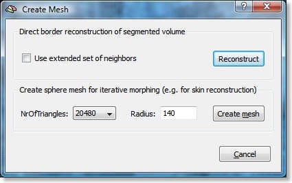
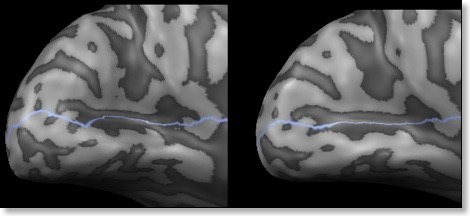
Several improvements have been made for the upcoming 1.9.10 release of BV QX with respect to creation, morphing and manipulation of meshes. First, the quality of reconstructed meshes has been improved by including more neighbors per vertex (a vertex is a 3D point usually connected to other mesh points). In previous versions, each vertex was connected to neighbors located in directions parallel to the cardinal axes (X, Y or Z). When turning on the new “Use extended set of neighbors” option in the “Create Mesh” dialog of 1.9.10, a vertex will be connected to additional neighbors, which are located in oblique directions. Due to the established denser neighborhood connectivity, more accurate morphing results can be achieved in subsequent steps, especially when performing distortion correction operations. Another advantage of the new meshes is that connections drawn from vertex to vertex are more accurately calculated, i.e. they follow more closely an intended connection path. This provides, for example, more straight lines when cutting a mesh for subsequent cortex flattening. The figure below shows a calcarine cut defined by a series of 5 points in 1.9.9 (left) and the obtained result obtained in 1.9.10 with the new mesh type and new path calculation routine (right).

In order to further increase precision, the code for selection of a vertex has been improved retrieving now the vertex which is closest to the point of a mouse click. In previous versions, the selected vertex returned after a click could be the second or third closest vertex instead. Note that also the logic to draw connected lines has been slightly changed. When a connected path is intended, the Shift key must be hold down from the first to the last mouse click. Clicking on a mesh without holding down the Shift key will highlight (mark) the closest vertex and never connects any points. This avoids unintended connections between end points of previous paths and newly started paths as could happen easily in previous versions.

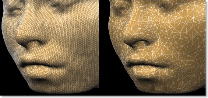
A disadvantage of the new meshes is that morphing operations run now slower as in previous versions due to the increased number of neighbors per vertex. If you experience the contrary effect, then you might use a modern computer with multiple cores and/or processors, which are now exploited due to implemented parallelized 3D morphing routines. Another possibility to increase speed would be to “simplify” a mesh by removing vertices, which are not strictly needed to represent the shape of a mesh. The figure on the top of this blog shows on the left side a head mesh, which was reconstructed with the usual sphere shrink-wrapping approach. In order to get a high-resolution starting mesh, I selected a sphere with 40962 vertices in the “Create Mesh” dialog instead of the default number of 20480 vertices. The right side of the figure shows a mesh with much less, but larger, triangles, which has been obtained by running the new mesh simplification routine introduced in 1.9.10, which can be called from the “Meshes > Mesh Simplification” menu item. This new tool allows to substantially reduce the number of vertices and triangles of a mesh by keeping the shape of the original mesh as intact as possible.

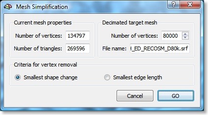
The “Mesh Simplification” dialog (see snapshot above) shows in the “Current mesh properties” field the number of vertices and triangles of a mesh before simplification. In the “Decimated target mesh” field, you may specify the number of vertices you want to have in the resulting simplified mesh. Mesh simplification proceeds in an iterative manner removing one vertex per iteration. In the “Criteria for vertex removal” field you may influence the strategy used to reduce (“decimate”) the number of vertices. If the “Smallest shape change” option is enabled, the vertex chosen for the next simplification step is the one which produces the smallest change in the shape of the mesh. When using the “Smallest edge length” option, the vertex chosen for the next simplification is the one which has a neighbor with the smallest distance of all mesh edges. Intuitively this strategy will also introduce minimal changes in the shape of the mesh but it might perform slightly worse than the strategy looking solely for minimal shape change. On the other hand, the “smallest distance” strategy results in meshes having more homogeneous distances between neighboring vertices, which might be relevant for some applications. The simplified head mesh in the figure on the top was created with the smallest shape change strategy and it shows that regions with high curvature (e.g. the tip of the nose or the lips) are not as strongly decimated as regions which are more flat. Both strategies allow to substantially reduce reconstructed head and cortex meshes without large shape modifications. This holds especially for the pattern of gyri and sulci of smoothed reconstructed (“RECOSM”) meshes, which are “oversampled” with many small triangles. The animation below shows the medial occipital region of a smoothed reconstructed cortex mesh and how it looks like after simplification from originally 134,797 vertices to meshes with 80,000, 40,000, 20,000 and 5,000 vertices.


Even when going down to 20,000 vertices, the rendered mesh looks almost indistinguishable from the originally rendered mesh. Only the mesh with 5,000 vertices, shows visible changes in the shape of the mesh.

In order to visualize the vertices and triangles clearly for the depicted images, a copy of the respected mesh is drawn as a wireframe on top of a shaded version of itself. In order to see the wireframe, it is also drawn slightly elevated with respect to the shaded version by moving each vertex slightly outward along its normal. In 1.9.10 you may produce these kinds of renderings simply by clicking the new “Draw Wireframe Over Shaded Mesh” item in the “Meshes > Rendering” menu.

The new possibility to simplify meshes opens a number of interesting applications in 1.9.10 and future versions of BrainVoyager QX:

• Fast animation of meshes. When using simplified versions of head and cortex meshes, it is possible to interact in real-time with these 3D representations even on computers with poor graphics hardware. This is especially relevant for the TMS Neuronavigator because real-time interactions with multiple meshes (e.g. two cortex hemisphere meshes plus a head mesh) is desirable during neuronavigation. In previous versions, simplified cortex meshes could only be created via the detour of sphere creation and sphere-to-sphere mapping. The new simplification routine allows a user to obtain simplified meshes in a minute with a simple button click.
• Modest simplification for fast and accurate morphing. Experience with cortex meshes with different amounts of simplification have shown that reducing the number to about 80,000 vertices does not reduce the quality of cortex inflation and flattening or cortex sphere creation but reduces calculation time significantly. Modest simplification has also no impact on visualization of statistical surface maps. This is expected when considering the mean distance between neighboring vertices, which is about 0.8 - 0.9 in original meshes, 1.0 - 1.1 in meshes simplified to 80,000 vertices and about 1.5 for meshes with 40,000 vertices. These numbers clearly indicate that even cortex meshes reduced to 40,000 vertices will properly sample volume time course data and statistical maps with voxel resolutions of 2 x 2 x 2 mm or lower. Note also that less vertices lead to more powerful statistics due to the reduced number of tests in the context of MTC-based statistics (this is not relevant for statistics after cortex-based alignment, since cortex meshes are standardized to 40962 vertices by using the sphere-to-sphere mapping approach). As a good compromise of very high quality and speed, I would suggest to create cortex meshes with 80,000 vertices, which is the default number of target vertices in the “Mesh Simplification” dialog for reconstructed meshes.
• Multiple-resolution meshes. In future versions of BV QX the mesh file format could be extended to store multiple versions of the same mesh with different complexity. When showing a mesh stationary, the highest resolution could be displayed while a simplified version could be shown when rotating and zooming it. Multi-resolution meshes are often used in 3D computer games in order to select a mesh with an appropriate complexity depending on the distance of the mesh to the observer.
• EEG / MEG continuous source modelling. Individual cortex meshes are helpful constraints to model EEG / MEG data at the source level, Various “minimum norm estimation” (MNE) techniques attempt to “project” channel data measured at electrodes or sensors to the underlying source space. The originally reconstructed cortex meshes in BrainVoyager QX possess too many vertices for these algorithms. With the possibility now to create almost arbitrarily simplified versions of cortex meshes retaining the shape of gyri and sulci as good as possible, MNE techniques can be applied more efficiently. The “Smallest edge length” option described above has been implemented with this application in mind.

Since meshes might now come in various versions, BV QX writes information about a mesh in the Log tab after loading. This information contains information on the type of mesh, the number of its triangles, vertices and edges and the average number of neighbors linked to a vertex as shown in the following example:

// Mesh "/CG2_3DT1FL_SINC4_TAL_LH_ED_RECOSM.srf" loaded
// Type: Reconstructed with extended set of neighbors
// # vertices: 134797
// # triangles: 269596
// average # of neighbors: 7.99993
// # edges: 539176, mean length: 0.870598, 0.0105843 - 1.86167